G-FOLD

SHIPLOG #0007 T+2120-05-09T11:52:46.205839

Now comes the moment of truth. I’m plummeting towards the planet and I need a way to make sure my craft can touch down safely. The obvious answer here is to fire my engine at maximum until my speed goes below some safe value (say 5 m/s), but this would be incredibly inefficient and use all my fuel up too early. I need a way to get as close to my landing position as possible while using as little fuel as possible. Not only that, but I need to ensure that this calculation can be done quickly as I’ll need to run it with whatever my actual position is in real time! This is no easy task, but luckily…there’s a solution.

Convexify

This type of problem is known as the soft landing problem. It can be expressed as a mathematical trajectory optimization problem where we optimize a discrete trajectory subject to a few constraints. The standard optimization has a lot of pieces, I won’t go into all the details (they can be found in the linked paper [1]), but here’s the general idea:

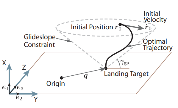
What this is trying to do is generate an optimal trajectory (given some initial position and velocity) that get’s as close to the target point as it can while following a few constraints. Namely it should stay in a cone with its tip at the landing point; this helps ensure the spacecraft doesn’t run into any nearby terrain obstructions (like a mountain). There are more constraints that are captured in the mathematical version of this optimization problem:

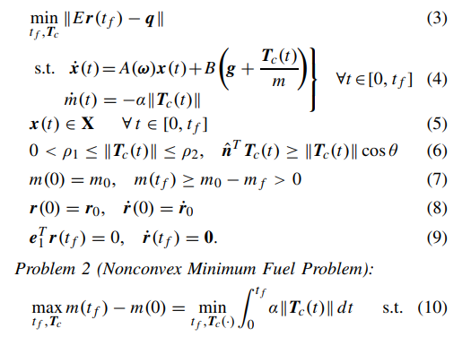
This problem is finding the closest landing position to the goal that it can while obeying some constraints. Namely:

• (4) This is a state space representation of the system dynamics which the ship must follow. Very similar to what was covered in the orbital trajectory solver.
• (5) The ship cannot exceed some maximum velocity I define and has to stay within a glide cone I define during it’s descent.
• (6) thrust has some minimum and maximum bounds as certain engines are only capable of some minimum and maximum, and the thrust pointing angle from vertical must be less than some arbitrary angle I pick \(\theta\). This helps keep the ship movements at a minimum and also keeps it from flipping upside down.
• (7) can’t use more fuel than the ship has
• (8) I have some start position and velocity
• (9) My end altitude and velocity should be

These are hard constraints that absolutely must be true, but the problem also specifies an objective. (10) is an objective that says to follow these constraints while using the least amount of fuel possible. The first part of the problem exchanges the fuel saving metric with a position metric however, minimizing the distance to the goal.

Once this problem finds the nearest target, a second iteration of this problem is done, but with a new constraint and the fuel objective. The new constraint is that it has to land at least as close as the first problem found a solution for, and the new objective is to minimize the mass loss instead of the distance to a goal point. The final time \(t_f\) can also be optimized by running the second solution through a line search until a best mass solution is found.

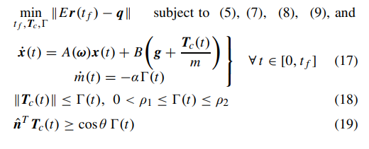
As defined, this problem is non-convex. So what does that mean? Well the short answer is that any function that is convex only has one single solution. This unique attribute means there are a lot of ways to cleverly solve this function and to do so quickly (that’s an entire field in and of itself so I won’t get into it here). In this case, the nonconvex parts of our problem are the lower thrust limit, the thrust divided by the mass and the thrust vector pointing condition. Fortunately there is a way to convert this to a convex problem!

It looks very similar and uses most of the same constraints, but some of the thrust elements have been replaced by \(\Gamma\) which ends up basically being equivalent to the magnitude of the thrust through some clever math. The convex solution ensures that, even though the constraints say \(\|\textbf{T}_c(t)\| <= \Gamma(t)\) it ends up actually being equal. Not shown is that thrust is replaced by a control variable \(\textbf{u}\) that is just the thrust vector divided by the mass. It basically cheats out the “thrust/mass” problem by considering it as one variable (the acceleration). Finally the mass is replaced with the natural log of the mass which ensures the new thrust constraints can remain convex. There are more variable changes, but I won’t go into them here (they can be found in [1]) as they’re fairly involved, but my hope is that this can at least give a vague idea of what the problem is trying to do.

Code!

Fortunately there’s a very nice package for solving these kinds of problems that follows the mathematical form closely (I’m using cvxpy). The first thing to do is to set up the problem variables and convenient ways to intialize them as they are described in [1]:

GFoldConfig = namedtuple('GFoldConfig', ['isp', 'm', 'm_fuel',
                                         'p1', 'p2',
                                         'g', 'pointing_lim', 'landing_cone',
                                         'q', 'v_max', 'w'])


_e1 = np.array([1, 0 ,0]).T
_e2 = np.array([0, 1 ,0]).T
_e3 = np.array([0, 0 ,1]).T
_E = np.array([[0, 1, 0], [0, 0, 1]])


def create_S(w):
    S = np.array([[0, -w[2], w[1]],
                  [w[2], 0, -w[0]],
                  [-w[1], w[0], 0]])
    return S

def create_A(w):
    S = create_S(w)
    A = np.zeros((6, 6))
    A[0:3, 3:6] = np.eye(3)
    A[3:6, 0:3] = -np.square(S)
    A[3:6, 3:6] = -2*S
    return A

def create_B():
    B = np.zeros((6, 3))
    B[0:3, :] = np.eye(3)
    return B

def get_cone(cone_angle):
    # cone angle between 0 and pi/2
    return _e1 / np.tan(cone_angle)

Then I’ll block out the actual problem itself. This function solves the GFOLD problem and returns the trajectory:

import cvxpy as cvp


def solve_gfold(config, start_pos, start_vel, iterations=100):
    dt = cvp.Parameter(1)  # There's a lot more to picking a delta t value, but this is mostly fine for a lot of landing problems for now
    x_0 = cvp.Parameter(6)

    x = cvp.Variable((6, N))  # N points along the trajectory x[0:3, k] is the position and x[3:6, k] is the velocity at each point
    u = cvp.Variable((3, N))  # Thrust vector control 
    gam = cvp.Variable(N)     # Thrust magnitude
    z = cvp.Variable(N)       # Natural log of the mass

    constraints = []
    constraints += set_boundary_constraints(constraints, config, x, u, gam, z, iterations, x_0) 
    constraints += set_path_constraints(constraints, config, x, u, gam, z, iterations, x_0)
    obj = cvp.norm(x[0:3, N-1] - config.q[:])  # Minimize the error between the goal and the landing position
    problem = cvp.Problem(cvp.Minimize(obj), constraints)
    problem.solve()

    return x.value

And now for the meat of the problem, setting up the constraints. This is where things get a little trickier to follow, but hopefully they look very similar to the original paper.

def set_initial_constraints(constr, config, x, u, gam, z, N, x_0):
    constr += [x[:, 0] == x_0[:]]   # Initial velocity and position
    constr += [x[3:6, N-1] == np.array([0, 0, 0])]  # Final velocity == 0

    # TODO (make initial thrust direction a parameter)
    constr += [u[:, 0] == gam[0]*_e1] # Initial thrust is vertical
    constr += [u[:, N-1] == gam[N-1]*_e1] # final thrust is vertical (or 0)
    constr += [z[0] == cvp.log(config.m)] # Initial mass

    constr += [x[0, N-1] == 0]  # Final altitude should be 0
    constr += [x[0, 0:N-1] >= 0]  # All altitudes during flight should be above the ground
    return constr

def set_path_constraints(constr, config, x, u, gam, z, dt, N):
    A_w = create_A(config.w)
    alpha = 1.0 / (config.isp * 9.8)
    pointing_angle = np.cos(config.pointing_lim)
    p1 = config.p1
    p2 = config.p2
    v_max = config.v_max
    c = get_cone(config.landing_cone)
    g = config.g

    # Simple Euler integration
    for k in range(N-1):
        # Rocket dynamics constraints
        constr += [x[0:3, k+1] == x[0:3, k] + dt*(A_w@x[:, k])[0:3]]  # System dynamics for the position
        constr += [x[3:6, k+1] == x[3:6, k] + dt*(g + u[:, k])]  # System dynamics for the velocity
        constr += [z[k+1] == z[k] - dt*alpha*gam[k]]  # System dynamics for the mass

        constr += [cvp.norm(x[3:6, k]) <= v_max]  # Velocity remains below maximum
        constr += [cvp.norm(u[:,k]) <= gam[k]]  # Helps enforce the magnitude of thrust vector == thrust magnitude
        constr += [u[0,k] >= pointing_angle*gam[k]]  # Rocket can only point away from vertical by so much
        constr += [cvp.norm(_E@(x[:3,k] - x[:3,-1])) - c.T@(x[:3, k] - x[:3,-1]) <= 0]  # Stay inside the glide cone

        if k > 0:  # There are a lot of tricks here to convexify the problem
            z_0 = cvp.log(config.m - alpha * p2 * (k) * dt)
            z_1 = cvp.log(config.m - alpha * p1 * (k) * dt)

            sigma_lower = p1 * cvp.exp(-z_0) * (1 - (z[k] - z_0) + (z[k] - z_0))
            sigma_upper = p2 * cvp.exp(-z_0) * (1 - (z[k] - z_0))

            # Minimimum and maximum thrust constraints
            constr += [gam[k] <= sigma_upper]
            constr += [gam[k] >= sigma_lower]
            # Minimum and maximum mass constraints
            constr += [z[k] >= z_0] 
            constr += [z[k] <= z_1]
    return constr

Now technically that only solves the first part of the landing problem, the position optimal part. There’s 2 more parts to GFOLD; the mass optimal problem and optimizing the final time (tf) to get the best mass usage. I won’t cover that here, but the mass optimal problem is very similar, however the objective changes to minimizing the final mass and it adds an extra boundary constraint on the final position. From there a line search on the tf variable can be done to find the tf that optimizes mass.

Really though, the position optimal problem is all that’s really required for this simple project, so for now I’m sticking to that. The beauty of this problem is that, despite how complex it seems, the convex solver solves it in a few milliseconds.

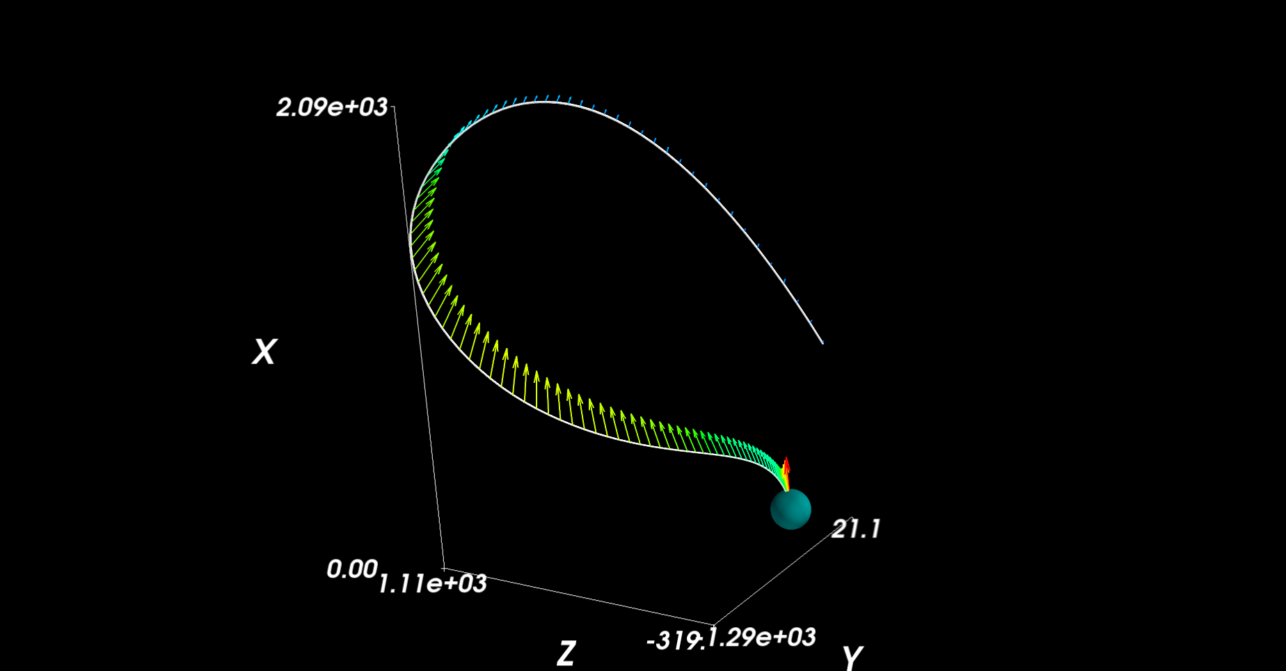
So running this gets some pretty cool results. Here’s one landing a test ship on top of the space center in KSP:

You can see how the trajectory generation compensates for the fact that the ship has momentum and limited thrust as it takes some time to bring it back around in the right direction. It also lands it nicely in the location I wanted, but this isn’t always the case. Following the constraints is far more important.

Of course this just generates a trajectory, it doesn’t actually follow it. Now I could just use the generated u values, but that will quickly diverge from the correct trajectory. This is because certain elements aren’t modelled in this problem, namely drag. But I can create a simple controller to follow it as best as possible. Once that’s done, I’m home free.

-/EOT/ - MC

Additional Resources

[1]http://www.larsblackmore.com/iee_tcst13.pdf - the GFOLD paper I used to generate the code for landing [2]https://www.matthewpeterkelly.com/research/MatthewKelly_IntroTrajectoryOptimization_SIAM_Review_2017.pdf - A good primer on how to set up optimization problems. Includes nonlinear optmization overview as well. [3]https://www.cvxpy.org/ - the python library for convex optimization