Eyes On
Author’s Note: This post touches on some more complicated subjects, including optics, vector fields, fourier transforms, and statistics.
SHIPLOG #0004 T+2120-05-07T13:24:39.2130184
I’ve got the ships camera systems up and running and can pull images from the downward facing camera on the ship. The next thing I want to do is find a good landing position. But the big question I have to ask, is what makes a good landing spot? Here are the big ones:
- Near the equator - this will be warmest, and on a cold planet like this one, that’s vital
- Near decent resources - any water below the surface will be of great help to me
- Reasonably flat - this one is probably the most important. I want to give my ship the best chances of landing.
Determining the proximity to the equator is trivial, and I can analyze resources with my ships hyperspectral cameras. The big open question is how to determine how flat the terrain is? Well that’s where things get a little more complicated.
Using Light
There are a lot of ways to extract 3D information about the surface. But I’m too high up and my camera doesn’t have a high enough resolution to use standard stereo approaches. However, utilizing some known characteristics about lighting I can reconstruct an approximation of the height of the surface and use that to determine how flat it is.
This is all built off of an assumption that the surface material is consistent and reflection of light on the surface is purely Lambertian. This means that the surface reflects in many directions with the brightest direction being directly normal to the surface. Basically I’m assuming the surface isn’t shiny.
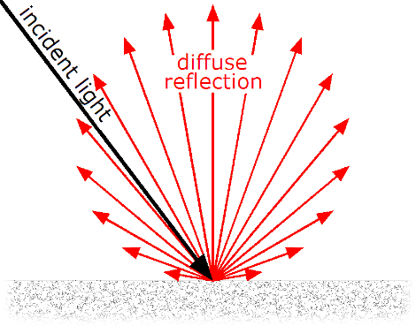
One interesting thing to note (hopefully clear from this image) is that the observed brightness doesn’t depend on the viewer! Only on the angle between the light and the surface. The equation for how this lighting works looks like:
\[I_{D}=\mathbf {L} \cdot \mathbf {N} \rho I_{L}\]where:
- \(I_{D}\) - the intensity of the reflected light
- N - the normal vector of the surface
- L - the light direction vector
- \(\rho\) - the albedo of the surface
- \(I_L\) - the intensity of the incoming light
This basically says the reflected light intensity is proportional to the angle between the lighting vector and the normal vector of the surface it’s illuminating.
We can make a generalized equation then for an image:
\[E(x, y) = \frac{\rho}{\sqrt{1 + p^2 + q^2}} [i_x i_y i_z] [-p, -q, 1]^T\]where:
- E(x, y) - the pixel brightness at position x, y (all images in grayscale)
- \(\rho\) - the albedo of the surface, assumed constant
- p, q - the x and y surface gradient, this is a mathematically convenient way to describe the normal vector
- \(i_x, i_y, i_z\) - the lighting vector (the magnitude of which is the light intensity)
In case you’re wondering where the square root part came from, the normal vector can be defined as:
\[n = \frac{1}{\sqrt{1 + p^2 + q^2}} [-p, -q, 1]^T\]What I’m really after here is p and q. Together, these tell me the angle of the surface at any point, and that’s the important data I need to know to determine how flat the suface is.
Author’s Note: while there are ways to estimate the direction and intensity of the light source as well as the albedo of the surface, I won’t go into that in this post. If you are interested, the code for doing this is included in the repo below.
Getting Depth
So how do we get the depth as well as the p and q values? Well there is an approach known as the Pentland approach that accomplishes that task. The first step is to convert the generalized equation into:
\[E(x, y) = \frac{psin(\sigma)cos(\tau) + qsin(\sigma)sin(\tau) + cos(\sigma)}{\sqrt{1 + p^2 + q^2}}\]The numerator is just the dot product of the lighting and surface gradient represented with trig functions. We also drop the albedo term because it’s constant everywhere and doesn’t affect integration. The taylor expansion of these terms can be used to simplify this equation down to:
\[E(x, y) \approx cos(\sigma) + pcos(\tau)sin(\sigma) + qsin(\tau)sin(\sigma)\]This helps remove the square root below and makes the math a little nicer. This means this is an approximation, but it’s a pretty good one.
Here is where the Fourier transform comes into play. Fourier Transforms have a lot of neat properties, but one of the most interesting ones are their ability to solve partial differential equations. Let’s start with the fourier transform of p and q being the partial derivatives of the surface, Z.
\[\mathcal{F} (p = \frac{\partial}{\partial x}Z(x, y)) = (-j\omega_x F_z({\omega}_x, {\omega}_y))\] \[\mathcal{F} (q = \frac{\partial}{\partial y}Z(x, y)) = (-j\omega_y F_z({\omega}_x, {\omega}_y))\]Taking the fourier transform of the simplified image equation (E(x, y)), substituting these equations for the fourier of p/q, and solving for F_z yields:
\[F_z(\omega_x, \omega_y) = \frac{F_E}{-j\omega_x cos\tau sin\sigma - j\omega_y sin\tau sin\sigma}\]Where \(F_E\) is the fourier transform of the image intensity. Z then just becomes the inverse fourier transform of that function. Now to code it up!
def estimate_surface_fft(self, image, filter_window=13):
    E = image / np.max(image)  # Assume the image is grayscale
    albedo, slant, tilt, I = self.estimate_lighting(image)
    Fe = scipy.fft.fft2(E)
    x, y = np.meshgrid(E.shape[1], E.shape[0])
    wx = (2*np.pi*x) / E.shape[0]
    wy = (2*np.pi*y) / E.shape[1]
    Fz = Fe / (-1j * wx * np.cos(tilt) * np.sin(slant) - 1j * wy * np.sin(tilt) * np.sin(slant))
    Z = np.abs(scipy.fft.ifft2(Fz))
    Z[Z == np.inf] = 0
    Z[Z == np.nan] = 0

    Z /= np.max(np.abs(Z))  # need to normalize as the final scale is on the order of 1e8
    p, q = np.gradient(Z)
    return Z_filtered, p, q
(Note that this has an estimate lighting function. I don’t cover that here, but if the lighting direction and albedo aren’t known there are ways to extract that information. It’s in the paper below[1] as well as in the code below[2])
I’ve taken a nice photo of the terrain below:

And running it through the analyzer gives me a depth output:

It looks pretty good! But there are some obvious issues that are shortcomings of this type of approach. Namely, it doesn’t handle shadows well, thinking they are steep inclines or declines, and there are ambiguities. Is that a crater? Or is it the top of a volcano? Even for humans it’s hard to tell so this program has trouble reconstructing it as well. Luckily, I don’t really care about that! What I really want is the surface normal which should be correct (for the most part). To turn this surface normal into something useful is a very straightforward process. For each pixel I take the surrounding neigbors and compute the variance from vertical. I then merely sum these variances to get a relative comparison metric for how uneven the terrain is. The result basically tells me how ‘noisy’ the terrain is.
The code is as follows:
def rolling_window(a, window):
    # This is a convenient way to run arbitrary functions on windows in a 2D array.
    shape = a.shape[:-1] + (a.shape[-1] - window + 1, window)
    strides = a.strides + (a.strides[-1],)
    return np.lib.stride_tricks.as_strided(a, shape=shape, strides=strides)

def variance_window(p, q, window_size=13):
    x_win = rolling_window(p, window_size)
    x_var = np.var(x_win, axis=-1)
    y_win = rolling_window(q, window_size)
    y_var = np.var(y_win, axis=-1)
    summed_var = x_var + y_var
    return summed_var
This results in the following with blue being more flat regions and yellow being more uneven:

Excellent! So the edges of the crater/volcano are especially uneven, but there are some nice flat spots inside of the crater/volcano and there’s a nice flat plane in the upper right of the image that’s in the same plane as my orbit. I have a landing spot! That plane in the upper right looks great. Next step, calculate an initial burn to land me there.
-/EOT/ - MC
Sources
[1] http://www.sci.utah.edu/~gerig/CS6320-S2015/Materials/Elhabian_SFS08.pdf - where a lot of information and code for these approaches was pulled from. An incredibly helpful primer. [2] https://github.com/heidtn/ksp_autopilot/blob/master/image_analyzer.py - the code to perform this reconstruction