Navigation Online
Author’s Note: If you haven’t read the first article ‘taking control’ on interfacing with the spacecraft, do that now. I’m using python numpy for the matrix math and mayavi for the plotting. Both can easily be installed with pip. I assume you know about vector math and a little about partial differential equations.
SHIPLOG #0003 T+2120-04-07T23:23:42.299564
I can now communicate with the ship’s base sensors and actuators. Problem is, the data coming from the ship is pretty simple. Raw data mostly, but with a little math and ingenuity, I can make this into something incredibly useful.
The ship sensors can tell me where I am relative to the planet, but in order to land this ship, I need to know where I’m going. A little knowledge of orbital mechanics is all it takes to turn basic information into something that will keep me alive. Speaking of where I’m going, I don’t have a name for this place other than ‘the planet’. I was thinking ‘Semot’, from an old Latin word that means ‘way the hell out there’. Fitting.
Now that my adversary is named, it’s time to get started.
Orbits 101
It turns out, there isn’t a lot of data needed to plot basic orbits. A long time ago, a smart guy called Newton figured it all out. He formulated Newton’s Law of Universal Gravitation:
\[g = G \times \frac{M}{r^2}\]Where:
- g - Acceleration due to gravity
- G - G is the gravitational constant
- r - The distance to the planet
- M - The mass of the planet
This says that if I know my position and the mass of the planet (both of which I get from my sensors) then I can calculate how quickly I’m accelerating towards the planet.
So how do I figure out the rest? Well let’s look at what I know: I know my current position, current velocity, and I can calculate the accelerations acting on our spacecraft at any point using my known current position. What I really want to try to figure out is what my next position is going to be some time from now. This inclues a differential equation that can be difficult to solve analytically. However solving the equation numerically is a sraightforward process. One easy way to solve this with the available information is to perform Euler integration. The basic concept is simple:
\[x_{t+\Delta t} = x_{t} + \Delta t x'_{t}\]Where:
- x - My position
- x’ - The derivative of my position, my velocity
- t - The current time
- \(\Delta t\) - (delta t) An arbitrarily small amount of time
So if I know my current position and I want to calculate my position some small delta t later, I can multiply my velocity by that small delta t and add it to my current position which will give me a prediction for my next one! This only is true if my velocity is linear, but for small enough delta t it works really well.
However, I don’t yet know what my velocity is supposed to be, after all it’s changing over time too, due to gravity. Well, it turns out I can do the same thing for my velocity! The derivative of my velocity is my acceleration, and the only thing accelerating my ship right now, is gravity which I now know how to calculate without needing any more derivatives.
So if y is my position, y’ is my velocity, and y’’ is my acceleration, I get the following equations:
\[x_{t+\Delta t} = x_{t} + \Delta t \times x'_{t}\] \[x'_{t+\Delta t} = x'_{t} + \Delta t \times x''_{t}\] \[x''_{t} = G \times \frac{M}{r^2}\]In software, I can then create a loop that first finds the next time step and then iterate on this new position I just calculated. Euler integration isn’t incredibly accurate, but it’s more than sufficient for my task and it’s simplicity makes it very convenient. Alternatives would be runge-kutta integration, ODE45, and even trapezoidal integration.
This is all one dimensional though, and I want to plot everything in three dimensions. Fortunately the same math extends easily to vectors without major changes. The only change is the following to Newton’s Universal Law:
\[x''_{t} = G \times \frac{M}{r^2} \hat{\mathbf{r}}\]The addition here is to add a unit vector \(\hat{\mathbf{r}}\) that points towards the center of gravitation. In this case, that’s just the center of the planet. Normalizing my position vector and flipping it will give me this unit vector.
Time to put it all together in some code:
from collections import namedtuple
import numpy as np
from mayavi.mlab import points3d, plot3d
from mayavi import mlab

OrbitConfig = namedtuple("OrbitConfig", ["mu", "planet_radius"])

class SimulateOrbit:
    def __init__(self, config):
        self.mu = config.mu  # KRPC uses mu which is just G*M in the Law of Universal Gravitation
        self.planet_radius = config.planet_radius  # I add the planet radius as an input so I can plot it

    def run_simulation(self, start_position, start_velocity, dt=1, iterations=100000):
        position = np.array(start_position)  # Position is a vector [Px, Py, Pz]
        velocity = np.array(start_velocity)  # Velocity is a vector [Vx, Vy, Vz]
        positions = []
        velocities = []

        for i in range(iterations):
            acceleration = self.get_gravity(position)	# Only the position is required to calcualte gravity
            velocity += acceleration * dt  # Euler integration on the velocity
            position += velocity * dt  # Euler integration on the position
            positions.append(np.array(position))
            velocities.append(np.array(velocity))

        return np.array(positions), np.array(velocities)

    def get_gravity(self, position):
        distance_from_center = np.linalg.norm(position)  # Pythagorean theorem yields the distance from the center
        gravitational_acceleration = self.mu / distance_from_center**2.0  # Calculate Newton's Law of Universal Gravitation
        # This is where things get a little harder to understand, the acceleration due to gravity has a direction, this direction
        # is pointed from the spacecraft towards the center of the planet.  We can use the position vector which points the other way
        # and just multiply it by negative 1 to flip the direction towards the planet.
        unit_position = position / distance_from_center
        gravity_vector = -1 * unit_position * gravitational_acceleration
        return gravity_vector

     def plot_positions(self, position_array, animate=False):
        f = mlab.figure(bgcolor=(0, 0, 0))
        points3d([0], [0], [0], scale_factor=self.planet_radius*2.0, resolution=128, color=(0, 0.5, 0.5))  # Plot the planet
        tube_size = self.planet_radius / 100.0	# Scale the trajectory line thickness so it shows up in the plot.
        s = plot3d(position_array[:, 0], position_array[:, 1], position_array[:, 2], tube_radius=tube_size, colormap='Spectral')
        mlab.show()
Not too long, thankfully. I’ve explained my process in the comments for the code. Now’s probably a good time to start on my autopilot system:
import krpc
import calculate_orbit

class AutoPilot:
    def __init__(self):
        self.conn = krpc.connect()
        self.vessel = self.conn.space_center.active_vessel
        self.body = self.vessel.orbit.body

    def print_name(self):
        name = self.vessel.name
        print(f"the vessel's name is: {name}")

    def print_position_and_velocity(self):
        p, v = self.get_position_and_velocity()
        print(f"Position: {p}\nVelocity: {v}")

    def get_position_and_velocity(self):
        position = self.vessel.position(self.body.orbital_reference_frame)
        velocity = self.vessel.velocity(self.body.orbital_reference_frame)
        return position, velocity

    def plot_orbit(self):
        p, v = self.get_position_and_velocity()
        config = self.get_orbit_config()
        orbit_simulator = calculate_orbit.SimulateOrbit(config)
        positions, velocities = orbit_simulator.run_simulation(p, v)
        orbit_simulator.plot_positions(positions)

    def get_orbit_config(self):
        mu = self.body.gravitational_parameter
        radius = self.body.equatorial_radius
        config = calculate_orbit.OrbitConfig(mu=mu, planet_radius=radius)
        return config
And all it takes to plot the orbit on live data from my spacecraft:
    autopilot = AutoPilot()
    autopilot.plot_orbit()

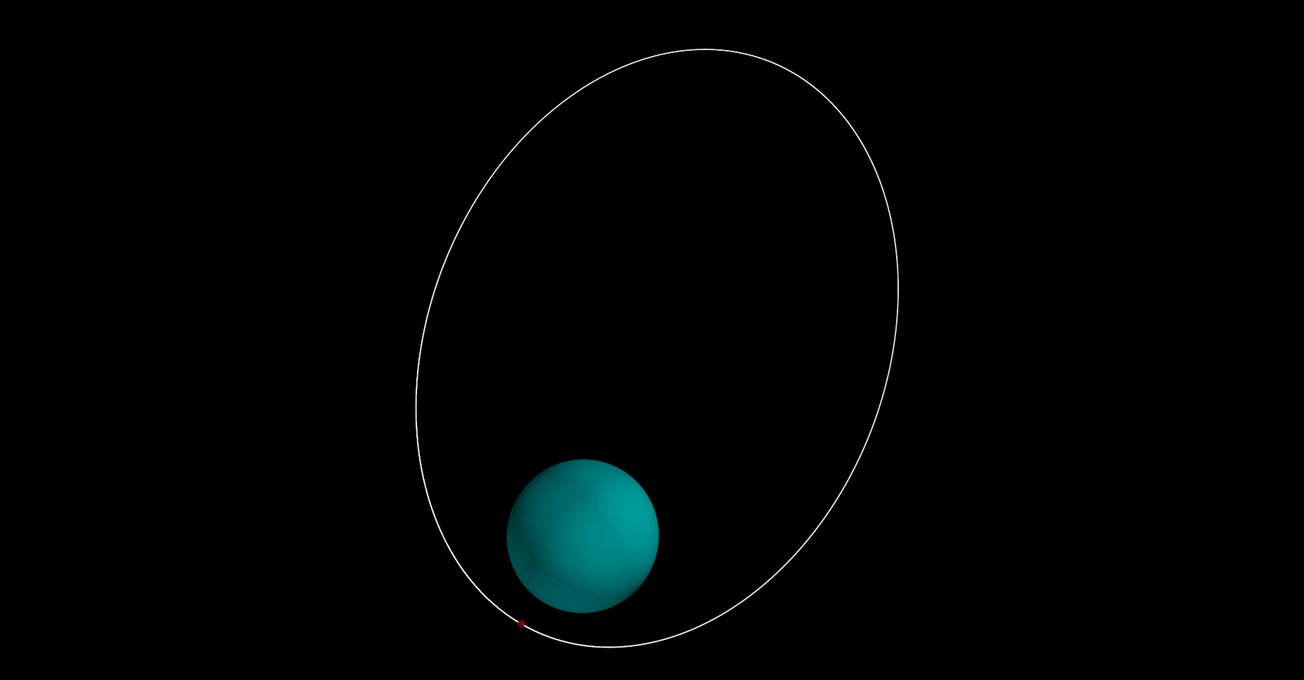
And there I am. Also there I go. That’s a pretty high orbit, and I’m not sure I have enough fuel to do a full landing. I’m going to have to aerobrake.
Bit of a drag
By dipping the ship just a bit into the atmosphere I can slow down enough for a landing. But my current model doesn’t tell me how the atmosphere will affect my spacecraft. I’m going to need to add drag forces into the equation to determine my decelleration. The drag equation is as follows:
\[F_D = \frac{1}{2} C \rho A v^2\]Where \(F_D\) is the force due to drag, C is the coeffecient of drag \(\rho\) is the desnity of the medium, A is the cross section area exposed to the drag forces, and finally v is the current velocity. Adding this into my model doesn’t take a whole lot of work with the Euler method, but getting some of these constants does. C can be figured out experimentally which I’ve done using my spacecraft simulator (plugging values into ksp until my predicted path matches my actual), A is assumed to be the area of the spacecrafts circular section, and we know v for any given time. \(\rho\) is a little harder, but thankfully kRPC handles that calculation for me. I’ll update the SimulateOrbit class to take in the new constants and calculate our drag.
OrbitConfig = namedtuple("OrbitConfig", ["mu",
                                         "planet_radius",
                                         "cross_section_area",
                                         "drag_coefficient",
                                         "density_function",
                                         "ship_mass"])


class SimulateOrbit:
    def __init__(self, config):
        self.mu = config.mu
        self.planet_radius = config.planet_radius
        self.cross_section_area = config.cross_section_area
        self.drag_coefficient = config.drag_coefficient
        self.density_function = config.density_function  # This is just a function pointer to the kRPC function call to get the density at an altitude
        self.ship_mass = config.ship_mass  # We need the ship mass to convert drag force to drag decelleration (F=ma)

    def run_simulation(self, start_position, start_velocity, dt=1, iterations=100000):
        position = np.array(start_position)
        velocity = np.array(start_velocity)
        positions = []
        velocities = []

        for i in range(iterations):
            acceleration = self.get_gravity(position) + self.get_drag(position, velocity) # Simply adding the two decelerations is enough.
            velocity += acceleration * dt
            position += velocity * dt
            positions.append(np.array(position))
            velocities.append(np.array(velocity))
            if np.linalg.norm(position) < self.planet_radius:	# Stop the simulation if we hit the planet!
                break

        return np.array(positions), np.array(velocities)

    def get_drag(self, position, velocity):
        v_mag = np.linalg.norm(velocity)  # pythagorean theorem to get the magnitude of our velocity
        density = self.density_function(position)  # Call the kRPC density function
        drag_force = 0.5 * density * self.drag_coefficient * self.cross_section_area * v_mag**2.0  # Calculate the drag force
        drag_decelleration_mag = drag_force / self.ship_mass  # Convert drag force to a deceleration using Newton's 2nd law: F=ma
        # This is where things get a little more complicated again, the direction of the drag force is opposite the direction of motion
        # i.e. the opposite direction of the velocity.  We do a similar trick to the gravity acceleration to calculate the drag
        # deceleration vector direction.
        v_unit_vec = velocity / v_mag
        drag_decelleration_vec = -v_unit_vec * drag_decelleration_mag
        return drag_decelleration_vec
And of course, an update to the autopilot to account for these new additions.
CROSS_SECTION_AREA = 5.381
COEFFICIENT_OF_DRAG = 1.455

class AutoPilot:
    """PREVIOUS CODE STILL HERE"""
    def get_orbit_config(self):
        mu = self.body.gravitational_parameter
        radius = self.body.equatorial_radius
        cross_section_area = CROSS_SECTION_AREA
        drag_coefficient = COEFFICIENT_OF_DRAG
        ship_mass = self.vessel.mass
        ref_frame = self.body.orbital_reference_frame
        # We have to do some tricks with the density function to make it
        # simple for our orbital calculator.  We make it so it defaults
        # to the orbital reference frame and our calculator no longer
        # needs to worry about reference frames.
        density_function = lambda x: self.body.atmospheric_density_at_position(x, ref_frame)
        config = calculate_orbit.OrbitConfig(mu=mu, planet_radius=radius, cross_section_area=cross_section_area,
                                             drag_coefficient=drag_coefficient, density_function=density_function,
                                             ship_mass=ship_mass)
        return config
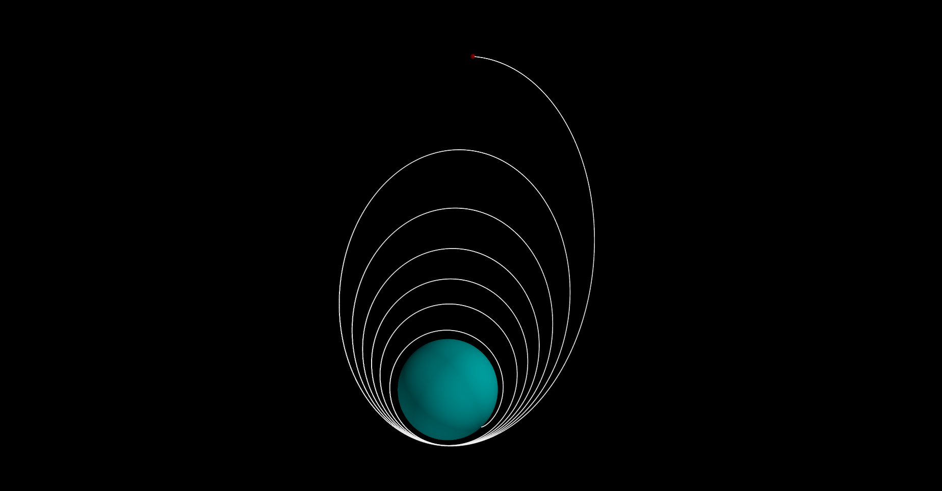
Et Voila. I’ll do a quick test burn at apogee to ensure everything’s working.

The next step is to find a good place to land and an initial burn that will put me close to that spot.
-/EOT/ - MC